Data Types

Adapted from http://changingminds.org/explanations/research/measurement/types_data.htm

There are four types of data that may be gathered in social research, each one adding more to the next. Thus ordinal data is also nominal, and so on.

Ratio Interval Ordinal Nominal

Nominal

The name 'Nominal' comes from the Latin nomen, meaning 'name' and nominal data are items which are differentiated by a simple naming system.

The only thing a nominal scale does is to say that items being measured have something in common, although this may not be described.

Nominal items may have numbers assigned to them. This may appear ordinal but is not -- these are used to simplify capture and referencing.

Nominal items are usually categorical, in that they belong to a definable category, such as 'employees'.

Example

The number pinned on a sports person.

A set of countries.

Ordinal

Items on an ordinal scale are set into some kind of order by their position on the scale. This may indicate such as temporal position, superiority, etc.

The order of items is often defined by assigning numbers to them to show their relative position. Letters or other sequential symbols may also be used as appropriate.

Ordinal items are usually categorical, in that they belong to a definable category, such as '1956 marathon runners'.

You cannot do arithmetic with ordinal numbers -- they show sequence only.

Example

The first, third and fifth person in a race.

Pay bands in an organization, as denoted by A, B, C and D.

Interval

Interval data (also sometimes called integer) is measured along a scale in which each position is equidistant from one another. This allows for the distance between two pairs to be equivalent in some way.

This is often used in psychological experiments that measure attributes along an arbitrary scale between two extremes.

Interval data cannot be multiplied or divided.

Example

My level of happiness, rated from 1 to 10.

Temperature, in degrees Fahrenheit.

Ratio

In a ratio scale, numbers can be compared as multiples of one another. Thus one person can be twice as tall as another person. Important also, the number zero has meaning.

Thus the difference between a person of 35 and a person 38 is the same as the difference between people who are 12 and 15. A person can also have an age of zero.

Ratio data can be multiplied and divided because not only is the difference between 1 and 2 the same as between 3 and 4, but also that 4 is twice as much as 2.

Interval and ratio data measure quantities and hence are quantitative.  Because they can be measured on a scale, they are also called scale data.

Example

A person's weight

The number of pizzas I can eat before fainting

Parametric vs. Non-parametric

Interval and ratio data are parametric, and are used with parametric tools in which distributions are predictable (and often Normal).

Normal (or Gaussian) distribution

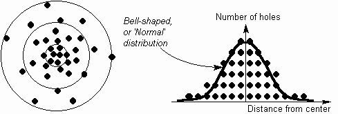
It is common in processes for most measurements to cluster around a central value, with less and less measurements occurring further away from this center. For example, the distribution of holes across the target will gradually spread out from a central, most common placement, as below.

The bell-shaped curve occurs surprisingly often and is consequently called a Normal distribution (or Gaussian distribution, after its discoverer, or simply Bell-curve) and has some very useful properties which can be used to help variation be understood and controlled.

Nominal and ordinal data are non-parametric, and do not assume any particular distribution. They are used with non-parametric tools such as the Histogram.

Histogram

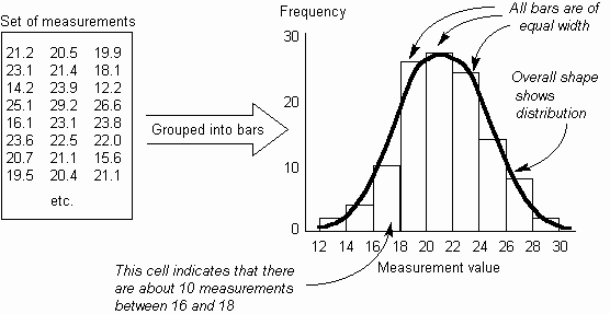
When measuring a process, it often occurs that the measurements vary within a range of values. By understanding how these measurements vary, the effects of the process and changes made to it can be better understood.

The Histogram shows the frequency distribution across a set of measurements as a set of physical bars. The width of each bar is constant and represents a fixed range of measurements (called a cell,bin or class). The height of each bar is proportional to the number of measurements within that cell. Each bar gives a solid visual impression of the number of measurements in it and together the bars show the distribution across the measurement range. The distribution of measurements can be seen far more clearly in the Histogram than in a table of numbers.

Continuous and Discrete

Continuous measures are measured along a continuous scale which can be divided into fractions, such as temperature. Continuous variables allow for infinitely fine sub-division, which means if you can measure sufficiently accurately, you can compare two items and determine the difference.

Discrete variables are measured across a set of fixed values, such as age in years (not microseconds). These are commonly used on arbitrary scales, such as scoring your level of happiness, although such scales can also be continuous.